Using a Streamline Model

This module calculates the streamline model using the formalism of Mendoza et al. (2009). This module was created for the Pineda et al. (2020) paper. A different tools to create and visualize the streamline model are available in the PIMS package, this package uses the original implementations from velocity_tools but with a nice visualization option.

The model calculates the streamline model under the influence of gravity from the central region (constant throughout the calculation), where the parcel of gas starts at a given position (radius, and spherical angles: theta and phi). This trajetory is further rotated by the inclination and position angle to obtain a trajectory that can be directly compared with the data.

Setting up the streamline model

In this implementation, the x-axis corresponds to -(RA), the z-axis to Dec, and the y-axis to the line of sight. This is an example of how to setup the streamline model:

import os
import matplotlib.pyplot as plt
from velocity_tools import stream_lines
from astropy import units as u
from astropy.wcs import WCS
from astropy.coordinates import SkyCoord, FK5
from astropy.visualization.wcsaxes import WCSAxes
from astropy.io import fits
plt.ion()
#
Per2_c = SkyCoord("3h32m17.92s", "+30d49m48.03s", frame='fk5')
Per2_ref = Per2_c.skyoffset_frame()

distance = 300
file_TdV = 'Per-emb-2-HC3N_10-9_TdV.fits'
# The file can be downloaded from:
if not os.path.isfile(file_TdV):
    import urllib.request
    link_file = 'https://github.com/jpinedaf/NOEMA_streamer_analysis/raw/eb3908e651e00dc9f110a8e82304222b83bb51fe/data/Per-emb-2-HC3N_10-9_TdV.fits'
    urllib.request.urlretrieve(link_file, filename=file_TdV)

# Create the streamline model
theta0 = 130.*u.deg
r0 = 0.9e4*u.au
phi0 = 365.*u.deg
v_r0 = 0*u.km/u.s
omega0 = 4e-13/u.s
v_lsr = 7.05*u.km/u.s
inc = -43*u.deg
PA_ang = 130*u.deg
Mstar = 3.2*u.Msun
# these are the results in astronomical units
(x1, y1, z1), (vx1, vy1, vz1) = stream_lines.xyz_stream(
                mass=Mstar, r0=r0, theta0=theta0, phi0=phi0,
                omega=omega0, v_r0=v_r0, inc=inc, pa=PA_ang,
                rmin=5.5e3*u.au, deltar=1*u.au)
dra_stream = -x1.value / distance * u.arcsec
ddec_stream = z1.value / distance * u.arcsec
fil = SkyCoord(dra_stream, ddec_stream, frame=Per2_ref).transform_to(FK5)
# Load the data
hdu = fits.open(file_TdV)[0]
wcs_TdV = WCS(hdu.header)
# create figure
plt.close('all')
fig = plt.figure(1, figsize=(6, 6))
ax = WCSAxes(fig, [0.1, 0.1, 0.8, 0.8], wcs=wcs_TdV)
fig.add_axes(ax)  # note that the axes have to be explicitly added to the figure
im = ax.imshow(hdu.data, cmap='inferno',
               vmin=0, vmax=160.e-3)#, transform=ax.get_transform(wcs_TdV))
ax.scatter(Per2_c.ra, Per2_c.dec, marker='*', transform=ax.get_transform('world'),
    facecolor='white', edgecolor='black')
ax.plot(fil.ra, fil.dec,  color='black', transform=ax.get_transform('world'), linewidth=5)
ax.plot(fil.ra, fil.dec,  color='red', transform=ax.get_transform('world'), linewidth=2)
plt.show()

Example of streamline calculation using the xyz_stream function. The streamline is shown in red, while the star shows the central YSO.

How to determine PA and inclination

The position angle (PA) and inclination are two important parameters that define the orientation of the angular momentum vector, or the orientation of the rotation axis. As an initial guess, we recomend to use the information already available in the literature regarding the disk and outflow orientation.

The PA is the angle between the North and the outflow direction, or the minor axis of the disk. The inclination is the angle between the disk plane and the line of sight. The inclination is defined as 0 degrees for a face-on disk and 90 degrees for an edge-on disk. Usually

import numpy as np
import astropy.units as u
import matplotlib.pyplot as plt
from velocity_tools import stream_lines

# Initial test: change in PA for vector = showin x- and y-axes
x_x = 1.
y_x = 0.
z_x = 0.
x_y = 0.
y_y = 0.
z_y = 1.
PA_Angle1 = 45 * u.deg
inc_1 = 30.0 * u.deg
PA_Angle2 = 75 * u.deg
inc_2 = -30.0 * u.deg
x_x_new1, y_x_new1, z_x_new1 = stream_lines.rotate_xyz(x_x, y_x, z_x,
                                            inc=inc_1, pa=PA_Angle1)
x_y_new1, y_y_new1, z_y_new1 = stream_lines.rotate_xyz(x_y, y_y, z_y,
                                            inc=inc_1, pa=PA_Angle1)
x_x_new2, y_x_new2, z_x_new2 = stream_lines.rotate_xyz(x_x, y_x, z_x,
                                            inc=inc_2, pa=PA_Angle2)
x_y_new2, y_y_new2, z_y_new2 = stream_lines.rotate_xyz(x_y, y_y, z_y,
                                            inc=inc_2, pa=PA_Angle2)

if (y_y_new1 > 0):
    color1='red'
else:
    color1='blue'
if (y_y_new2 > 0):
    color2='red'
else:
    color2='blue'
# Plot x- and y-axes only
plt.ion()
plt.close('all')
fig1, ax1 = plt.subplots(figsize=(7,7))
ax1.plot([0, x_x], [0, z_x], color='black')
ax1.plot([0, x_y], [0, z_y], color='black')

ax1.plot([0, x_x_new1[0]], [0, z_x_new1[0]], color='k', ls='--')
ax1.plot([0, x_y_new1[0]], [0, z_y_new1[0]], color=color1, ls='--')

ax1.plot([0, x_x_new2[0]], [0, z_x_new2[0]], color='k', ls=':')
ax1.plot([0, x_y_new2[0]], [0, z_y_new2[0]], color=color2, ls=':')
ax1.axis('equal')
ax1.set_xlabel('x')
ax1.set_ylabel('y')
ax1.text(0.1, -0.1, f"PA = {PA_Angle1}, inc = {inc_1}", color=color1)
ax1.text(0.1, -0.2, f"PA = {PA_Angle2}, inc = {inc_2}", color=color2)
plt.show()

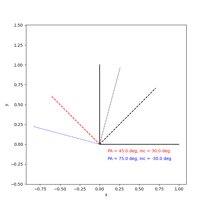
Example of how the position angle (PA) and inclination (inc) affect the orientation of the x- and z-axes. The solid lines show the original orientation, while the dotted and dashed lines show the new orientation after the rotations. The red line show the direction with red-shifted z-axis, while the blue line show the blue-shifted z-axis.

In the case of the streamline model, the goal is to place the x-axis pointing towards the red-shifted side of the disk, while the z-axis pointings towards outflow direction. The sign of the inclination angle is determined to match the color of the outflow (red or blue).